Library
library(here)
library(readxl)
library(tidyverse)
library(ggplot2)
library(scales)
library(drc)
library(gt)
theme_set(theme_bw())library(here)
library(readxl)
library(tidyverse)
library(ggplot2)
library(scales)
library(drc)
library(gt)
theme_set(theme_bw())data_0040 <-
readxl::read_excel(here("data_raw/data_0040/CE.LIQ.FLOW.062_Tidydata.xlsx"))
data_0040 %>% head() %>% gt::gt()| plateRow | plateColumn | vialNr | dropCode | expType | expReplicate | expName | expDate | expResearcher | expTime | expUnit | expVolumeCounted | RawData | compCASRN | compName | compConcentration | compUnit | compDelivery | compVehicle | elegansStrain | elegansInput | bacterialStrain | bacterialTreatment | bacterialOD600 | bacterialConcX | bacterialVolume | bacterialVolUnit | incubationVial | incubationVolume | incubationUnit | incubationMethod | incubationRPM | bubble | incubateTemperature |
|---|---|---|---|---|---|---|---|---|---|---|---|---|---|---|---|---|---|---|---|---|---|---|---|---|---|---|---|---|---|---|---|---|---|
| NA | NA | 1 | a | experiment | 3 | CE.LIQ.FLOW.062 | 2020-11-30 | Sergio Reijnders - Ellis Herder | 68 | hour | 50 | 44 | 24157-81-1 | 2,6-diisopropylnaphthalene | 4.99 | nM | Liquid | controlVehicleA | N2 | 25 | OP50 | heated | 0.743 | 8 | 300 | ul | 1,5 glass vial | 1000 | ul | rockroll | 35 | NA | 20 |
| NA | NA | 1 | b | experiment | 3 | CE.LIQ.FLOW.062 | 2020-11-30 | Sergio Reijnders - Ellis Herder | 68 | hour | 50 | 37 | 24157-81-1 | 2,6-diisopropylnaphthalene | 4.99 | nM | Liquid | controlVehicleA | N2 | 25 | OP50 | heated | 0.743 | 8 | 300 | ul | 1,5 glass vial | 1000 | ul | rockroll | 35 | NA | 20 |
| NA | NA | 1 | c | experiment | 3 | CE.LIQ.FLOW.062 | 2020-11-30 | Sergio Reijnders - Ellis Herder | 68 | hour | 50 | 45 | 24157-81-1 | 2,6-diisopropylnaphthalene | 4.99 | nM | Liquid | controlVehicleA | N2 | 25 | OP50 | heated | 0.743 | 8 | 300 | ul | 1,5 glass vial | 1000 | ul | rockroll | 35 | NA | 20 |
| NA | NA | 1 | d | experiment | 3 | CE.LIQ.FLOW.062 | 2020-11-30 | Sergio Reijnders - Ellis Herder | 68 | hour | 50 | 47 | 24157-81-1 | 2,6-diisopropylnaphthalene | 4.99 | nM | Liquid | controlVehicleA | N2 | 25 | OP50 | heated | 0.743 | 8 | 300 | ul | 1,5 glass vial | 1000 | ul | rockroll | 35 | NA | 20 |
| NA | NA | 1 | e | experiment | 3 | CE.LIQ.FLOW.062 | 2020-11-30 | Sergio Reijnders - Ellis Herder | 68 | hour | 50 | 41 | 24157-81-1 | 2,6-diisopropylnaphthalene | 4.99 | nM | Liquid | controlVehicleA | N2 | 25 | OP50 | heated | 0.743 | 8 | 300 | ul | 1,5 glass vial | 1000 | ul | rockroll | 35 | NA | 20 |
| NA | NA | 2 | a | experiment | 3 | CE.LIQ.FLOW.062 | 2020-11-30 | Sergio Reijnders - Ellis Herder | 68 | hour | 50 | 35 | 24157-81-1 | 2,6-diisopropylnaphthalene | 4.99 | nM | Liquid | controlVehicleA | N2 | 25 | OP50 | heated | 0.743 | 8 | 300 | ul | 1,5 glass vial | 1000 | ul | rockroll | 35 | NA | 20 |
Column RawData has missing data in cells 192-196, or samples in vialNr 3, compName napthalene. These data points are NA in the data when loaded into R studio. Most compUnits use nM, Ethanol and S-medium use pct.
data_0040_tidy <- data_0040
data_0040_tidy$compConcentration <-
  as.numeric(data_0040$compConcentration)
Since compConcentration is of character type, the data does not get plotted properly and we change it to numeric.
# create ggplot, adding concentration to x-axis and measured data to y-axis
# control/experiment are defined by shape, components are defined by colour
data_0040_graph <-
  as_tibble(data_0040_tidy) %>%
  ggplot(aes(x = compConcentration,
             y = RawData,
             shape = expType,
             colour = compName)) +
  geom_point(position = position_jitter(w = 0.03, h = 0)) +
  scale_x_continuous(trans = log10_trans()) + # log10 scale is applied to make results more readable.
  labs(title = "Effect of compounds on C. elegans offspring") +
  ylab("Offspring Count") +
  xlab("Compound Concentration")
print(data_0040_graph)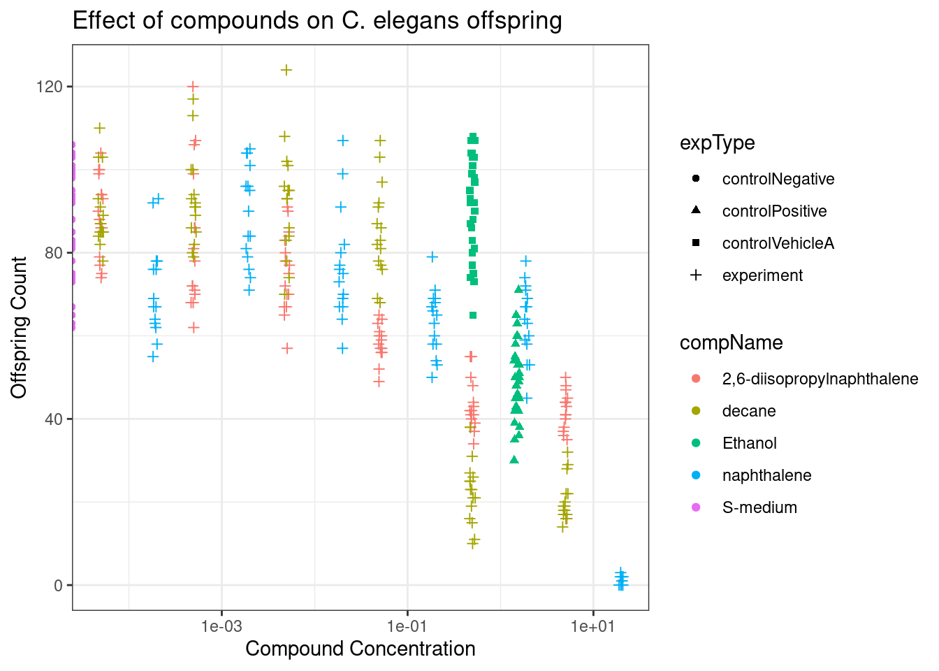
Figure 1 shows a scatter plot of the C. elegans offspring data after the adults have been incubated in differing concentrations of the different compounds; 2,6-diisopropylnapthalene, decane, napthalene, the positive control ethanol and the negative control S-medium. As the differences in concentrations were quite large, we changed to a log10 scale to more clearly present the data. We also added a slight jitter to the data points to displace each point and make it easier to read, as a lack of jitter results in a straight vertical line of data points.
# facet wrap to show individual graphs
data_0040_graph +
  facet_wrap(vars(compName))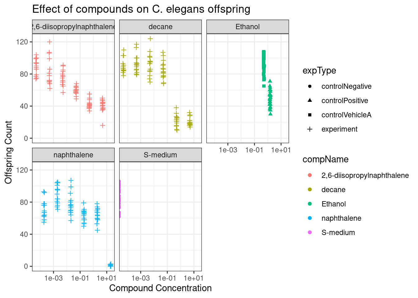
With the each component split into its own plot in Figure 2 using facet_wrap it is easier to see the downward trend in the offspring count once the concentration of the components increases.
# data is normalized for negative control by setting the mean of negative control to 1

negative_control_mean <- data_0040_tidy %>%
  filter(expType == "controlNegative") %>%
  summarise(mean_value = mean(RawData, na.rm = TRUE)) %>%
  pull(mean_value) # get the value from the mean_value in the tibble without having to use $mean_value

# normalize the data:
# if the data is negative control, set value to 1
# else divide raw data by negative control mean to create value as a fraction
data_0040_temp <- data_0040_tidy
data_0040_normalized <- data_0040_temp %>%
  mutate(
    NormalizedData = if_else(expType == "controlNegative", 1, RawData / negative_control_mean)
  )

# print normalized dataset as ggplot
data_0040_normalized_graph <-
  data_0040_normalized %>%
  ggplot(aes(x = compConcentration,
             y = NormalizedData,
             shape = expType,
             colour = compName)) +
  geom_point(position = position_jitter(w = 0.03, h = 0)) +
  scale_x_log10() +
  labs(title = "Effect of compounds on C. elegans offspring",
       subtitle = "Normalized data compared to negative control") +
  xlab("Compound concentration") +
  ylab("Normalized offspring count")
print(data_0040_normalized_graph)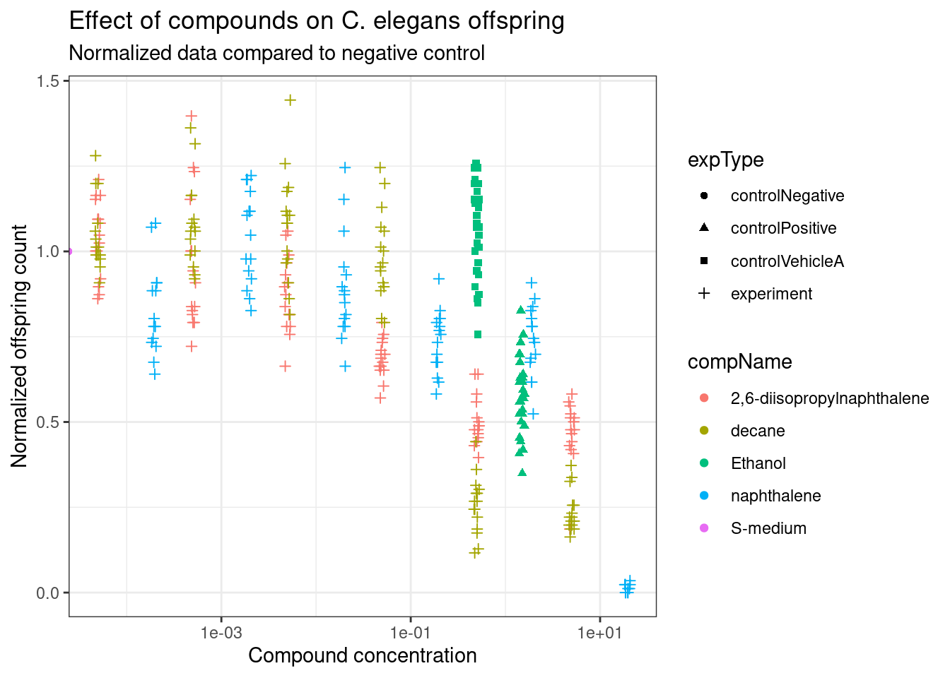
As the nematodes grow differently due to variance we have different amounts of offspring per adult. In Figure 3 the data has been normalized using the negative control as a baseline to show the impact of the compounds on the offspring count.
data_0040_filter_exp <- data_0040_tidy %>%
  filter(expType == "experiment")

# data_0040_filter_exp_naphthalene <-
#   data_0040_filter_exp %>%
#   filter(compName == "naphthalene")
#
# drm_nap <-
#   drm(data = data_0040_filter_exp_naphthalene,
#     formula = RawData ~ compConcentration,
#     fct = LL.4())
#
# plot(drm_nap, main = "naphthalene")

####

exp_compname <- data_0040_filter_exp$compName %>% unique()

for (i in exp_compname) {
  drm_calc <- drm(data = data_0040_normalized %>% filter(compName == i),
               formula = NormalizedData ~ compConcentration,
               fct = LL.4())

  plot(drm_calc,
       main = i,
       ylab = "Normalized Offspring Count",
       xlab = "Compound Concentration (nM)")

  # calc EC50 using ED, extract [1] ec50 value
  ec50 <- round(ED(drm_calc, 50)[1], digits = 2)

  # Add EC50 annotation to the plot
  abline(h = 0.5, lty = 2) # line hor at 0.5 offsprint count, line ver at ec50, lty dashed lines
  abline(v = ec50, lty = 2)
  text(x = ec50,
       y = 0.6,
       labels = paste("EC50: ", ec50, "nM"),
       pos = 2) # position left of point
}
Estimated effective doses

       Estimate Std. Error
e:1:50 0.025072   0.010998
Estimated effective doses

       Estimate Std. Error
e:1:50 0.119453   0.042934
Estimated effective doses

       Estimate Std. Error
e:1:50    3.129        NaN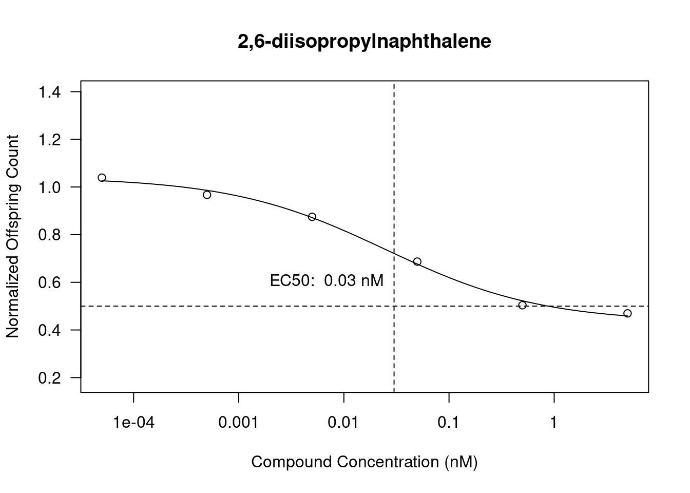
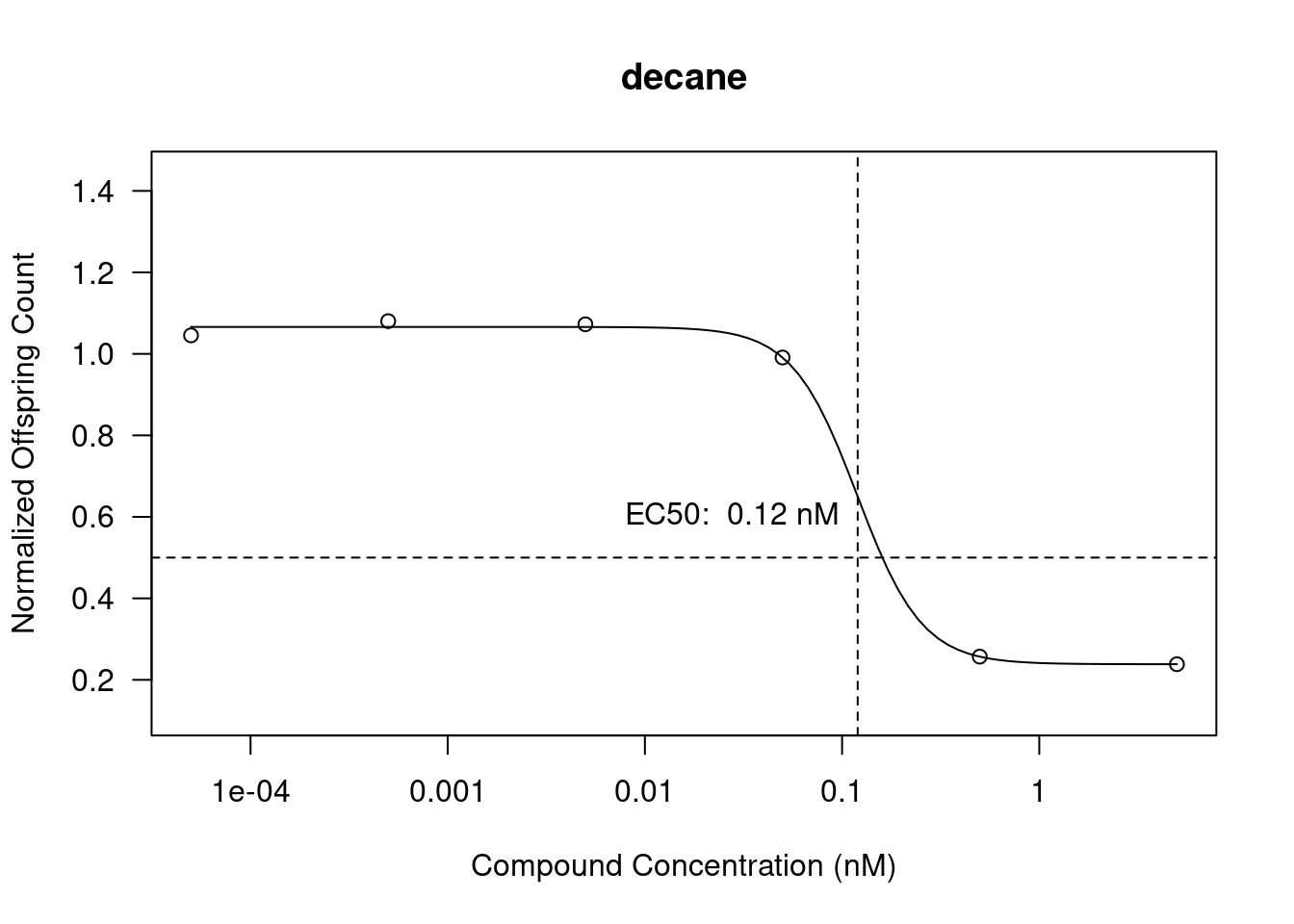
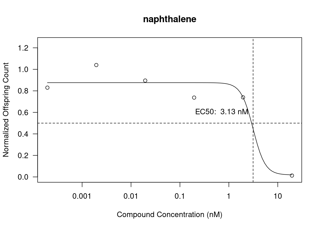
Dose response curves (DRCs) have been plotted using the drc package using the normalized offspring data and the compound concentrations. Using de ED function we also calculate the EC50 values and add them to the plots.
In Figure 4 (a) we see 2,6-diisopropylnaphthalene has an EC50 of 0.03 (nM) and the normalized offsrping count gradually goes down when the compound concentration goes up. The EC50 however doesn’t intersect with the graph properly as it should be more around the range of 0.49 (nM) following the line.
In Figure 4 (b) We see decane have an EC50 of 0.12 (nM). The graph shows a steep decrease in normalized offspring count after 0.0499 (nM). The calculated EC50 doesn’t quite intersect at the 50% as the compound concentration seems to be higher on the graph with 0.12 (nM) reaching about 60%.
In Figure 4 (c) we see naphthalene with an EC50 of 3.13 (nM). The offspring count has a steep decrease after about 1.95 (nM) of compound.